Contents
The signal model is a mathematical description of the signals received across a phased array. It accounts for the source directions, array geometry, relative phase shifts between antenna elements, source amplitudes, interference, and noise. For far-field sources, the incident wavefront is commonly approximated as a planar wave.
The signal model provides the foundation for understanding and deriving direction-of-arrival (DoA) estimation methods. It connects the physical propagation geometry with the complex samples measured by the array and explains how source direction is encoded in the spatial phase progression.
Snapshot Model
A snapshot is the vector of complex samples measured across all antenna elements at one observation instant.
For an array with $M$ antenna elements and $K$ incident sources, one snapshot is modeled as
$$ \mathbf{x} = \mathbf{A}\mathbf{s} + \mathbf{n}. $$
where
- $\mathbf{x} \in \mathbb{C}^{M \times 1}$ — received snapshot vector across the array,
- $\mathbf{A} \in \mathbb{C}^{M \times K}$ — array manifold matrix,
- $\mathbf{s} \in \mathbb{C}^{K \times 1}$ — complex source signal vector,
- $\mathbf{n} \in \mathbb{C}^{M \times 1}$ — additive noise vector.
The array manifold matrix is formed from the steering vectors of all incident sources:
$$ \mathbf{A} = \begin{bmatrix} \mathbf{a}(\theta_1) & \mathbf{a}(\theta_2) & \cdots & \mathbf{a}(\theta_K) \end{bmatrix}. $$
Each column $\mathbf{a}(\theta_k)$ describes the phase progression across the array for a source arriving from direction $\theta_k$.
import numpy as np

M = 8
angles_deg = [0, 30]
d_over_lambda = 0.5

m = np.arange(M)

# Array manifold matrix A
A = np.column_stack([
    np.exp(-1j * 2 * np.pi * d_over_lambda * m * np.sin(np.deg2rad(theta)))
    for theta in angles_deg
])

# Source vector s and noise n
s = np.array([1.0, 0.7 * np.exp(1j * np.deg2rad(40))])

rng = np.random.default_rng(7)
n = 0.1 / np.sqrt(2) * (
    rng.standard_normal(M) + 1j * rng.standard_normal(M)
)

# Snapshot
x = A @ s + n

np.set_printoptions(precision=2, suppress=True)

print("A =\n", A)
print("\ns =", s)
print("\nn =", n)
print("\nx = A @ s + n = ", x)
Steering Vector
A steering vector describes the complex response of the array to a planar wave arriving from a given direction. Its elements represent the relative phase shifts, and optionally amplitude variations, observed across the antenna elements for that direction.
A uniform linear array (ULA) consists of equally spaced receiving elements arranged along a straight line.
The distance between adjacent elements is the inter-element spacing $d$. The direction of arrival (DoA), denoted by $\theta$, is defined as the angle between the target direction and the normal to the array axis, also called the array broadside.
For a far-field target, the reflected signal is approximated as a planar wave. Because the wavefront reaches the antenna elements at different positions, each virtual channel observes a relative propagation delay and therefore a corresponding phase shift.
These phase shifts form the steering vector. For a ULA, the phase progression is approximately linear across the array, and its slope is determined by the target direction, the wavelength, and the inter-element spacing.
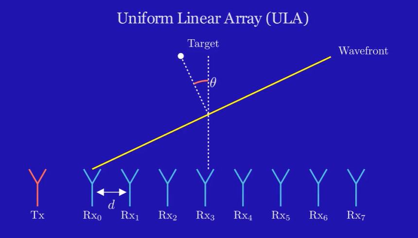
For a ULA with inter-element spacing $d$, the steering vector for a plane wave arriving from angle $\theta$ is
$$ \mathbf{a}(\theta) = \begin{bmatrix} 1 \\ e^{-jkd\sin\theta} \\ e^{-j2kd\sin\theta} \\ \vdots \\ e^{-j(M-1)kd\sin\theta} \end{bmatrix}, $$
where
- $M$ — number of antenna elements,
- $d$ — spacing between adjacent elements,
- $\theta$ — direction of arrival measured from broadside,
- $k = \dfrac{2\pi}{\lambda}$ — wavenumber,
- $\lambda$ — wavelength,
- $j = \sqrt{-1}$ — imaginary unit.
Equivalently, the $m$-th steering-vector entry is
$$ [\mathbf{a}(\theta)]_m = e^{-jmkd\sin\theta}, \qquad m = 0,1,\ldots,M-1. $$
For half-wavelength spacing, $d = \lambda/2$, the phase increment between adjacent elements becomes
$$ \Delta \phi = -\pi \sin\theta. $$
The plots show measured snapshots acquired with the AWR2243 radar for a single corner reflector placed approximately at $0^\circ$ broadside and $45^\circ$ off boresight.
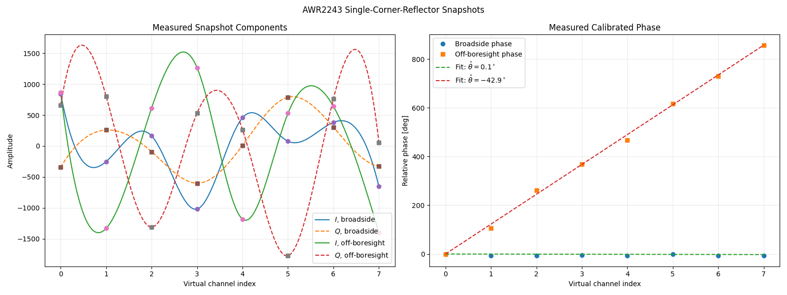
The I/Q components illustrate how the complex array response changes across the virtual channels. For the broadside reflector, the channel phases remain approximately aligned, while the off-boresight reflector produces a systematic rotation of the complex samples across the array.
The calibrated and unwrapped phase makes this spatial behavior more explicit. The broadside target produces a nearly constant phase progression and therefore a fitted slope close to zero. The off-boresight target produces an approximately linear phase ramp. The slope of this ramp is determined by the array geometry and is directly related to the target DoA.